Theory for Experimentalists

From lattice relaxation to DLTS-based extraction of NMP parameters.

This page is organized as a practical narrative for DLTS users: why a defect transition couples to lattice motion, how that modifies the capture or emission kinetics, why the familiar Arrhenius-like plot bends away from strict linearity, and how the full temperature dependence can be used to recover \( \omega \), \( \Delta Q \), and \( \Delta E \).

1. Lattice relaxation

2. Capture coefficient vs temperature

3. Curved \( \ln(T^2/e_n) \) plot

4. Parameter inversion

Part I

Lattice relaxation and configuration coordinate diagram

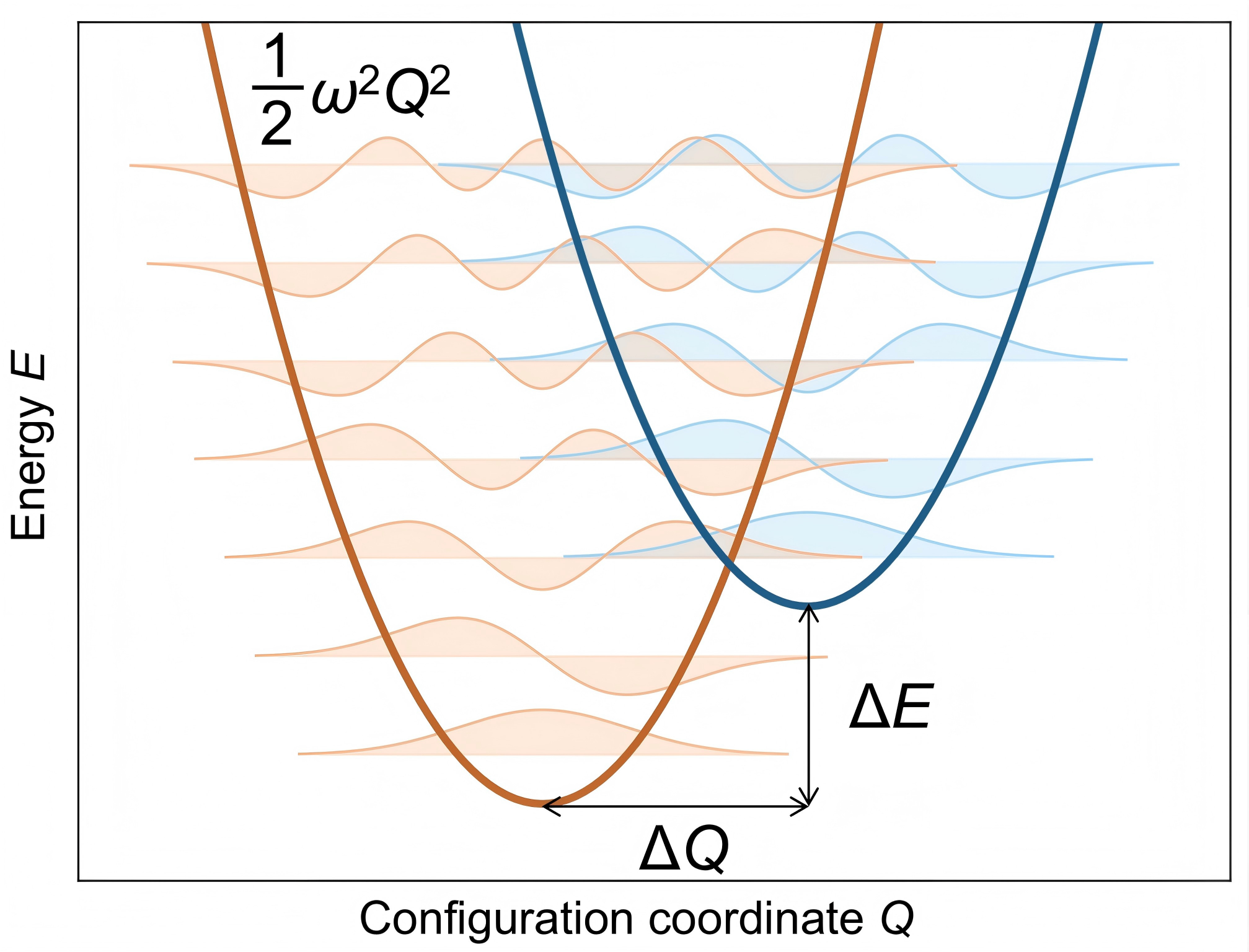
Carrier capture at defects probed by deep-level transient spectroscopy is a nonradiative multiphonon electronic transition. Defects capture or emit carriers and change the charge state, so the initial and final states are associated with different equilibrium configurations, with a displacement \( \Delta Q \) along the configuration coordinate diagram, which is usually referred to as lattice relaxation. Under a single-phonon-mode approximation, with a vibrational frequency \( \omega \), the potential energy surfaces are constructed under the harmonic approximation, where \( U = \frac{1}{2}\omega^2 Q^2 \). The two potential energy surfaces are then separated by \( \Delta Q \) horizontally and by \( \Delta E \) vertically, where \( \Delta E \) is the defect transition energy associated with the defect level.

References

Huang and Rhys, Proc. A 204, 406 (1950).
Henry and Lang, Phys. Rev. B 15, 989 (1977).
Huang, Contemp. Phys. 22, 599 (1981).

Figure Concept

Configuration coordinate diagram

Open Image

Part II

Carrier capture cross section as a combined temperature-dependent quantity

In practical DLTS analysis, the carrier capture cross section \( \sigma_n \) is not governed by a single temperature trend. Instead, it reflects the combined contributions from the NMP capture coefficient \( C_n \), the carrier thermal velocity \( v_{\mathrm{th}} \), and the Sommerfeld factor \( f_s \). The full cross section therefore follows \( \sigma_n = C_n / v_{\mathrm{th}} * f_s \).

The four panels below are placeholders for the final figures. They are laid out as one visual sequence so an experimental reader can immediately see how the individual temperature-dependent factors combine into the observed \( \sigma_n(T) \).

Component 1

NMP transition rate

\( r(T) \)

Component 2

Carrier thermal velocity

\( v_{\mathrm{th}}(T) \)

Component 3

Sommerfeld factor

\( f_s(T) \)

→

Combined Result

Carrier capture cross section

\( \sigma_n(T) \)

Part III

The DLTS plot no longer remains strictly linear

In a simplified picture, one often expects a straight line when plotting \( \ln(T^2/e_n) \) against \( 1000/T \). NMP theory predicts that the measured points can deviate systematically from this linear form. That curvature is not a nuisance. It is useful information about the defect-lattice coupling.

This section should help readers reinterpret curvature in DLTS-derived plots as a physically meaningful signature rather than merely an experimental imperfection.

Figure Concept

\( \ln(T^2/e_n) \) vs \( 1000/T \)

Part IV

Using the full curve to invert \( \omega \), \( \Delta Q \), and \( \Delta E \)

Workflow

From data points to parameter extraction

1 DLTS-derived data

\( e_n(T) \) or related temperature-dependent observables

→

2 NMP forward model

temperature-dependent rates generated from trial parameters

→

3 Inverse fit

best-fit \( \omega \), \( \Delta Q \), \( \Delta E \)

Once the departure from strict linearity is recognized as part of the physics, the natural next step is to fit the entire temperature dependence rather than a reduced linear surrogate. That is the motivation for the inversion workflow.

In this framework, the experimental points are compared against an NMP-based forward model, and the final goal is to extract the parameter triplet \( \omega \), \( \Delta Q \), and \( \Delta E \) that best explains the data.

This is the section where your final wording can connect the theory page to the fitting portal.